Geometric Brownian motion

A geometric Brownian motion (GBM) (also known as exponential Brownian motion) is a continuous-time stochastic process in which the logarithm of the randomly varying quantity follows a Brownian motion,^[1] also called a Wiener process. It is used in mathematical finance to model stock prices in Black–Scholes model.

1 Technical definition
2 Properties of GBM
3 Use of GBM in finance
4 Extensions of GBM
5 See also
6 References
7 External links

Technical definition

A stochastic process S_t is said to follow a GBM if it satisfies the following stochastic differential equation (SDE):

$dS_t = \mu S_t\,dt %2B \sigma S_t\,dW_t$

where $W_t$ is a Wiener process or Brownian motion and $\mu$ ('the percentage drift') and $\sigma$ ('the percentage volatility') are constants.

Properties of GBM

For an arbitrary initial value S₀ the above SDE has the analytic solution (under Itō's interpretation):

$S_t = S_0\exp\left( \left(\mu - \frac{\sigma^2}{2} \right)t %2B \sigma W_t\right),$

which is (for any value of t) a log-normally distributed random variable with expected value and variance given by^[2]

$\mathbb{E}(S_t)= S_0e^{\mu t},$

$\operatorname{Var}(S_t)= S_0^2e^{2\mu t} \left( e^{\sigma^2 t}-1\right),$

that is the probability density function of a S_t is:

$f_{S_t}(s; \mu, \sigma, t) = \frac{1}{\sqrt{2 \pi}}\, \frac{1}{s \sigma \sqrt{t}}\, \exp \left( -\frac{ \left( \ln s - \ln S_0 - \left( \mu - \frac{1}{2} \sigma^2 \right) t \right)^2}{2\sigma^2 t} \right).$

The correctness of this solution can be checked using Itō's lemma.

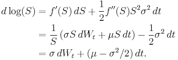
When deriving further properties of GBM, use can be made of the SDE of which GBM is the solution, or the explicit solution given above can be used. For example, consider the stochastic process log(S_t). This is an interesting process, because in the Black–Scholes model it is related to the log return of the stock price. Using Itō's lemma with f(S) = log(S) gives

$\begin{alignat}{2} d\log(S) & = f^\prime(S)\,dS %2B \frac{1}{2}f^{\prime\prime} (S)S^2\sigma^2 \, dt \\ & = \frac{1}{S} \left( \sigma S\,dW_t %2B \mu S\,dt\right) - \frac{1}{2}\sigma^2\,dt \\ &= \sigma\,dW_t %2B(\mu-\sigma^2/2)\,dt. \end{alignat}$

It follows that $\mathbb{E} \log(S_t)=\log(S_0)%2B(\mu-\sigma^2/2)t$ .

This result can also be derived by applying the logarithm to the explicit solution of GBM:

$\begin{alignat}{2} \log(S_t) &=\log\left(S_0\exp\left(\left(\mu - \frac{\sigma^2}{2} \right)t %2B \sigma W_t\right)\right)\\& =\log(S_0)%2B\left(\mu - \frac{\sigma^2}{2} \right)t %2B \sigma W_t. \end{alignat}$

Taking the expectation yields the same result as above: $\mathbb{E} \log(S_t)=\log(S_0)%2B(\mu-\sigma^2/2)t$ .

Use of GBM in finance

Main article: Black–Scholes model

Geometric Brownian Motion is used to model stock prices in the Black–Scholes model and is the most widely used model of stock price behavior.^[3]

Some of the arguments for using GBM to model stock prices are:

The expected returns of GBM are independent of the value of the process (stock price), which agrees with what we would expect in reality.^[3]
A GBM process only assumes positive values, just like real stock prices.
A GBM process shows the same kind of 'roughness' in its paths as we see in real stock prices.
Calculations with GBM processes are relatively easy.

However, GBM is not a completely realistic model, in particular it falls short of reality in the following points:

In real stock prices, volatility changes over time (possibly stochastically), but in GBM, volatility is assumed constant.
In real stock prices, returns are usually not normally distributed (real stock returns have higher kurtosis ('fatter tails'), which means there is a higher chance of large price changes).^[4]

Extensions of GBM

In an attempt to make GBM more realistic as a model for stock prices, one can drop the assumption that the volatility ( $\sigma$ ) is constant. If we assume that the volatility is a deterministic function of the stock price and time, this is called a local volatility model. If instead we assume that the volatility has a randomness of its own—often described by a different equation driven by a different Brownian Motion—the model is called a stochastic volatility model.

References

^ Ross, Sheldon M. (2007). "10.3.2". Introduction to Probability Models.
^ Oksendal, Bernt K. (2002), Stochastic Differential Equations: An Introduction with Applications, Springer, pp. 326, ISBN 3540637206
^ ^a ^b Hull, John (2009). "12.3". Options, Futures, and other Derivatives (7 ed.).
^ Wilmott, Paul (2006). "16.4". Paul Wilmott on Quantitative Finance (2 ed.).

External links

Geometric Brownian motion models for stock movement except in rare events.